Building HorizonDB in production
Radar powers location at scale. Our platform handles more than a billion API requests every day, supporting hundreds of millions of devices around the world.
In our previous blog post, How we replaced Elasticsearch and MongoDB with Rust and RocksDB, we shared the fundamental components of HorizonDB, our in-house geospatial database that powers our platform.
Today, we're excited to go under the hood and share part of the iterative engineering journey behind our search and geocoding APIs.
We'll talk about where the system stands today, and where it's headed next.
In this post we'll focus on two data structures that power HorizonDB: FST (finite state transducers) and Tantivy (inverted indices). We'll cover how our usages of these structures have shaped over time.
Building and scaling our system architecture
HorizonDB started as a month-long effort by engineers Jeff Kao and Bradley Schoeneweis. We were developing an address validation API.
From proof-of-concept to 2-tier architecture
We also wanted to explore using Quickwit's Tantivy library and RocksDB, so we scoped the project to support just well-structured address validation requests.
.png)
Early results were promising: competitive performance on commodity hardware, with a smooth development, build, and deploy experience. We decided to take the service into production for address validation, and later expanded it to handle a subset of forward geocoding traffic.
That rollout went well. To expand its surface area and support Regions and Places (points-of-interest) in forward geocoding, we built separate Tantivy indexes and RocksDB stores for Regions and Places data. This isolation begins at the data source level and continues through our data pipelines, into our indexes and data stores. This isolation also exists at the code-level, separating domain-specific logic, and at runtime, executing each clients' queries on concurrent threads.
We also built a ranking component to aggregate, score, and sort results from each client.
.png)
At this point, HorizonDB was handling about 20% of our total search traffic. To support autocomplete, we needed to improve both performance and precision for short, prefix-style inputs.
Every system has a few defining characteristics that shape its optimization path. For HorizonDB, the key was that 80% of our queries are well-formed.
For example, a typical US address looks like:[street number] [street] [unit] [city] [state] [postal code]
Region queries might be simpler, like:[city] [state] or [state] [country]
Tantivy's inverted index had served us well up to this point, but we saw an opportunity to add a lightweight prefix-matching layer to speed things up.
That led us to Andrew Gallant's FST crate, which let us cache millions of "happy paths" in just a few megabytes of memory. On an FST hit, we could return results an order of magnitude faster than a Tantivy query. We got to work adding a happy-path cache to each of our clients.
.png)
As we added an FST to each client, we saw a clear performance boost. p50 latency dropped, fleet CPU usage decreased, and we were able to serve the same traffic with fewer machines. That gave us confidence to begin routing a subset of autocomplete traffic to HorizonDB.
But we soon ran into a new bottleneck. Often, a query would hit one client's FST and return a good result in just a few milliseconds, but the request still had to wait for other clients to finish querying their own FSTs and fallback to Tantivy. For example, a query like "One Infinite Loop, Cupertino" might quickly match in the Address FST, but still wait on the Regions and Places clients.
We have addressed this in several ways, including building out query classification. But the system-level fix was to split the system into two tiers: a "fast" search tier powered by the FST, and a "deep" search tier powered by Tantivy. The fast tier is optimized for speed and precision, while the deep search tier optimizes for recall.
We added another ranking step after the fast path, along with logic to decide whether those results were good enough. This lets us run fast-path searches across all clients first and often return early, before falling back to deep search if needed.
.png)
The impact was significant. This architecture has held up over the past year as we've added query classification and tagging models, improved index usage, and matured our ranking system.
Ship, learn, expand
We didn't plan out this architecture on day one. Instead, it emerged from the problems we needed to solve. We might have designed it this way intentionally if we knew exactly what we needed, but discovery was part of the process. What I can say with certainty is that building it this way allowed us to derisk the entire effort and incrementally realize value on our engineering investment.
Soon after v1 was complete, HorizonDB was already serving a narrow slice of traffic. Each improvement allowed it to handle more traffic. The more real-world traffic it handled, and the more developer time we put in, the clearer the problem statement became: the constraints HorizonDB needed to operate within, what it needed to be a viable long-term investment, and where we could make domain-specific optimizations.
Because of that, there were very few risky, large-scale cutovers. We used traffic shadowing and API diff to maintain search quality while optimizing for performance. We rolled out changes in phases, kept a safety net in place, and gradually migrated endpoints off our legacy search stack.
In May 2024, a little over a year after we kicked off the project, we fully sunset our non-HorizonDB search infrastructure.
Of course, it wasn't as simple as just dropping data into these structures. In the next section, I'll share a few challenges we ran into when building the indexes, and how we resolved them.
Indexing 500M FST labels
Our initial FST builds had several performance hot spots. We resolved these issues through partitioning, custom automatons, motivated from simple query analysis.
The initial build
We explain some of how FSTs work in our previous HorizonDB post, but I’d also recommend Andrew Gallant's post, Index 1,600,000,000 Keys with Automata and Rust.
When we started building our first FSTs, we identified a set of common query shapes we wanted to support. A few examples:
And if you can imagine all the different ways people search for a place, I owe you a dollar.
Labels are cheap. Taking into account synonyms, city aliases, nearby cities with common landmarks, and other variations, we generated over 500 million labels to represent our dataset. We stored some basic metadata in the label's u64 value and tied each label to its underlying record by appending the record's internal ID, like this:
A query like "San J" would return all keys starting with "sanj". We do preliminary ranking and filtering based on metadata, parse out the best record IDs, and fetch full records from RocksDB for "deeper" ranking.
This initial strategy had some issues:
- Region name prefixes follow a power-law distribution. Common prefixes, like
"New"or"San", appear extremely often. - There are millions of unique postal codes worldwide. In countries like Canada, Brazil, and Ireland, there are unique postal codes per block.
- Postal code label variations comprised the bulk of our label space while actual postal code queries represented just a portion of our search volume.
- Due to our automaton implementation, we had to traverse every matching result before we could apply any filtering rules.
This all combined to create over-saturated portions of the FST and uneven query performance. A query for "Sao Paulo", ostensibly a query for the city, would trigger a traversal of 200k+ Sao Paulo city and postal code label combinations, with all the postal code records being tossed for being a poor match. Likewise, a query for "San J" would sift through hundreds of "San Jose" and "San Juan" labels from around the world, even if the query was targeting the US.

Relieving FST saturation
FST recall was too large based solely on prefix matches, especially when most candidates could be trimmed from simple country or region type checks.
We needed to apply that filtering earlier, so we prefixed all labels with the record's ISO-2 country code and, for Regions, with the region type (e.g. postal code, city, state).
This effectively created ~250 country-specific partitions in our FSTs, and a two-level partition in the Regions FST. We built a FST Automaton that:
- Parses the region type / country code.
- Prunes irrelevant branches.
- Forwards the rest to the standard StartsWith Automaton.
During query analysis, we determine whether the input likely includes a postal code. If it does, we include the postal code region type in our automaton filter.
.png)
Figure 6: Label structure with metadata prefixing. This example shows how "San Jose" and "San Juan" labels, along with postal codes, are partitioned by country and region type. Due to FST compression on both ends of the key, the underlying storage may not match this layout exactly.
Latency improved significantly. Even though we gave up some compression efficiency, we significantly reduced search space by applying basic filtering early.
This did not eliminate all hot spots, since cities like Dublin still have hundreds of unique postal codes. However, the increased performance overall gave us room to implement other performance improvements down the pipeline.
Wrangling street numbers in Tantivy
On the Tantivy side, we faced a performance issue in our address search implementation involving street numbers. Search performance was correlated with the street number attached to the query, with low street numbers doing especially poorly.
The initial build
In an inverted index, each term is linked to a postings list of documents that contain that term. For street, city, or state names, this works well because the number of unique terms is reasonably limited.
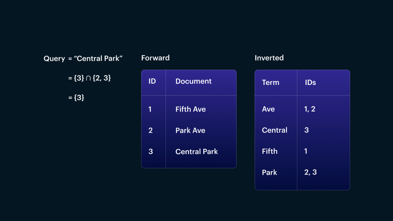
Figure 7: A query like "Central Park" can be handled efficiently by querying the terms "central" and "park" and combining the documents returned by each.
In our initial implementation, we used discrete street numbers as distinct terms in the inverted index. This had a few issues:
- The number of unique terms is HUGE, and most of those terms (ie:
"13721A") will point to a very small number of records. - The "uniqueness" of street numbers caused BM25 scoring (a variant of TF-IDF) to overweight the importance of street numbers.
- A mistyped street number (like
"123"instead of"124") would completely miss, making the system overly brittle.
We explored several solutions during HorizonDB's early development and eventually settled on one that made sense at the time: bucketing street numbers into ranges (like "0>50", "1000>2000") and indexing those ranges as terms in Tantivy.
This let us use street numbers in BooleanQueries like any other term, while introducing some built-in fuzziness. For example, a query for "123 Fake St" would require the "100>150" bucket term, surfacing results for "Fake St" even if the exact street number was not present.
.png)
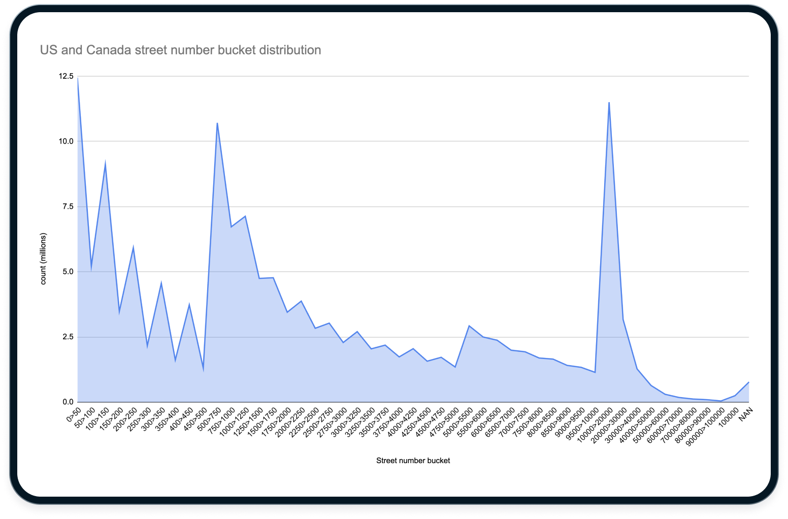
One of the primary considerations when designing the bucket range distribution was that street numbers in the US and Canada are not evenly distributed:
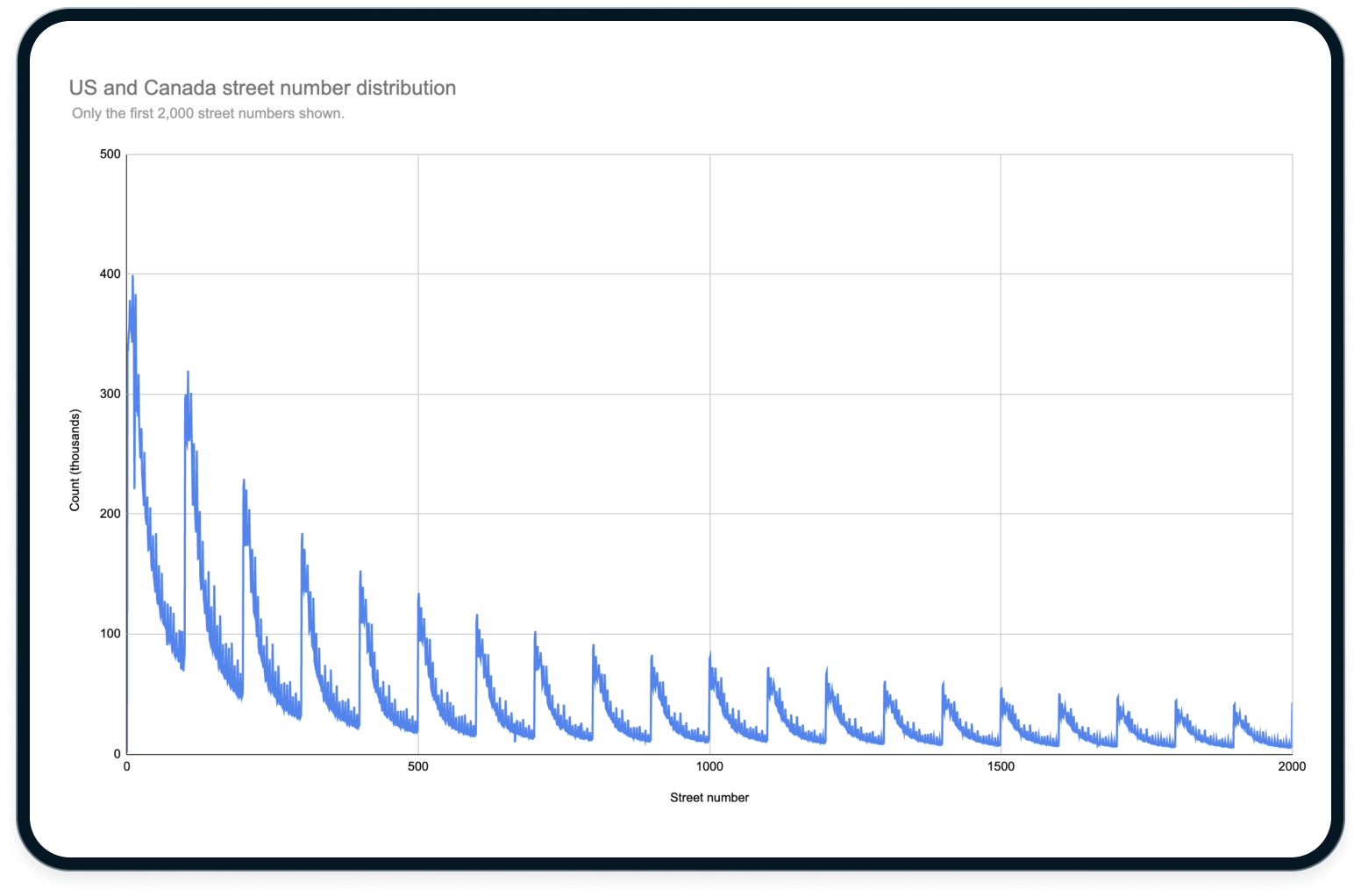
To create a more even distribution, we chose street number buckets that increased in size on a roughly logarithmic scale. This gave us smaller buckets at the low end and larger ones at the high end. This still produced some saturated spots but generally had an acceptable performance and recall profile.
Going international
This solution fell apart once we started indexing addresses outside the US and Canada. In global datasets, the contrast between low street numbers and the rest of the distribution is much more pronounced:

When we applied our existing bucket distribution to global data, the pseudo-log scale wasn't enough to partition the space effectively. About 60 percent of global street numbers fell into the 0–50 bucket, and 80 percent were below 250:
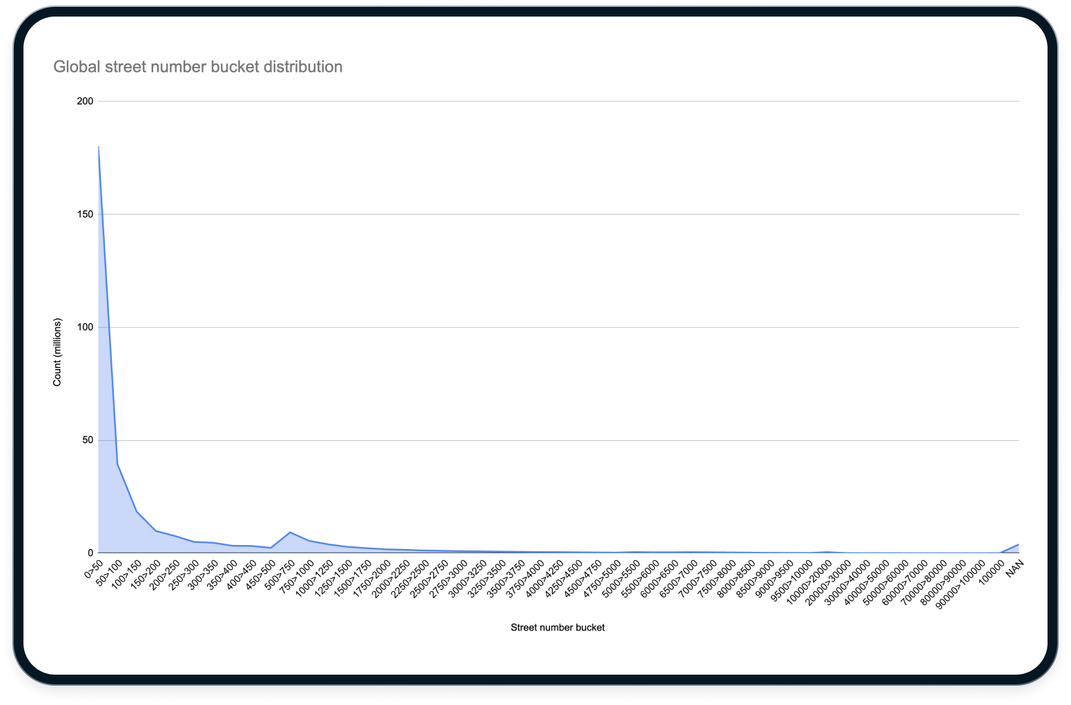
As a result, queries in those early buckets barely narrowed the search space. Queries with higher street numbers resolved quickly, while those with lower numbers took unacceptably long.
We experimented with a few different indexing and boolean query strategies before concluding that, because of their distribution, street number-derived terms were not a great candidate for inverted index terms. At least not the way we were doing it.
We needed to rethink our approach.
Using more of Tantivy's toolbox
After reviewing flamegraphs, we realized that Tantivy was doing too much aggregation and scoring work during those slow queries. We decided to offload some of that to a more direct filtering mechanism.
Inspired by Tantivy's FilterCollector, we represented each street's number buckets as a u64 bitmap. We stored that in a Tantivy fast field, allowing quick columnar access at collection-time. Because the 0-250 space was so saturated, we also stored each individual street number that the record had from that range in an additional four u64 fast field bitmaps.
We updated our query processing to build bitmasks for the street numbers and buckets parsed from the query.
We then implemented a Tantivy Collector that:
- Filters records by intersecting the query's street number bucket bitmask with each record's bitmap.
- Scores the remaining records using BM25.
- Boosts any record whose street-number bitmap shows an exact match within the 0–250 range.

This let us shift work out of Tantivy's BooleanQuery and Scorer, and move it to columnar lookups and bitmask checks. It improved precision where we needed it most, in the densest part of our street number distribution. As a result, we saw better precision, smoother p90+ latency, and more predictable performance across address workloads.
Wrapping it up
There's still a lot we haven’t covered here, and we're excited to dive deeper in future posts.
HorizonDB is also far from finished. We're continuing to make the system smarter, faster, and more accurate. Here are a few things we're working on right now:
- More advanced query classification using language models.
- Low level Tokio, RocksDB, and instance-level optimizations.
- Bespoke data structures that take more advantage of our highly structured datasets.
Join us
Radar is more than an API layer. Across SDKs, maps, databases, and infrastructure, we're rethinking geolocation from the ground up to build the fastest, most developer-friendly location stack out there.
If this post caught your interest, we're hiring engineers across the stack.
Check out our jobs page to learn more.